Gehört zu: Astrofotografie Software
Siehe auch: Plate Solving, AnSvr, Polar Alignment, APT, N.I.N.A.
Benutzt: Fotos aus pCloud
Stand: 02. Juni 2023
Astrofotografie mit der Software AstroTortilla
Zusammenfassung
Anwendungsbereich von AstroTortilla
Mit AstroTortilla kann man eine Kamera ansteuern und dann Plate Solving machen. Die Plate-Solving-Ergebnisse können als SYNC-Points (Alignment Points) zur Teleskopsteuerung verwendet werden. Dadurch funktioniert ein Goto ohne 3-Star-Alignment.
Gliederung
- Meine ersten Schritte
- AstroTortilla Tutorial
Meine ersten Schritte mit der Software AstroTortilla
Installation von AstroTortilla
Wenn man AstroTortilla auf Windows installiert, wird ganz automatisch das Cygwin mit installiert. Anscheinend benötigt das AstroTortilla um das API zu astronometry.net zu realisieren.
Setup einer Kamera in AstroTortilla
AstroTortilla möchte als erstes eine Kamera und als zweites ein Teleskop “haben”.
Als Kamera hat man folgendes zur Auswahl:
- Disconnected
- BackyardEOS
- Astro Photography (IP-Adress and Port)
- Screen Capture
- MaxIm DL
- ASCOM Camera
- File Open Dialog
- Nebulosity 2/3
Kamera-Setup als “ASCOM Camara”
Da ich gerade meine erste schicke AstroCam erstanden hatte (eine Altair GPCAMMT9M034M) und da auch etwas von ASCOM drauf stand, habe ich “ASCOM Camera” als erstes ausprobiert.
Als Basis benötigt man zu allerest die ASCOM-Platform. Auf der Web-Seite http://ascom-standards.org finde ich zum Download: ASCOMPlatform62.exe
Als zweites brauche ich den ASCOM-Kamera-Treiber. Den gab es auf der Herstellerseite: http://cameras.altairastro.com/
Wenn ich meinen Windows-Computer nun neu starte und dann zur Kontrolle SharpCap aufrufe, kann ich tatsächlich eine “Altair Astro Camera ASCOM Driver” im Dropdown sehen und wenn ich diese auswähle erscheint auch tatsächlich ein Bild – SUPER!
Auch in AstroTortilla kann ich jetzt unter “Camera” eine “ASCOM Camera” auswählen und komme dann nach dem Klicken auf den Setup-Botton auf den “ASCOM Camera Chooser” wo ich die “Atair Astro Camera ASCOM Driver” aussuchen kann.
Nachdem nun alles richtig eingestellt ist, könnte ich auf den Button “Capture and Solve” drücken, aber die Cam ist ja noch garnicht auf den Sternenhimmel gerichtet. Ich könnte aber bereits vorhandene Astro-Fotos zum Solven ausprobieren, in dem ich als Camera nicht die wirkliche Kamera angebe, sondern aus dem Kamera-Dropdown “File Open dialog” auswähle.
Kamera-Setup als “File Open dialog”
Aus dem Kamera-Dropdown haben wir nun “File Open dialog” ausgewählt. Der Setup-Button hat dann keine Funktion, aber wenn man jetzt auf den Button “Capture and Solve” drückt, kann man ein bereits vorhandenes Astrofoto auswählen, was dann “gesolved” wird…
Testfall #1
- Ich habe ein Foto ausgewählt: ShapCap Captures > 2016-04-17 > Capture > 22_45_53 > 0001.fits
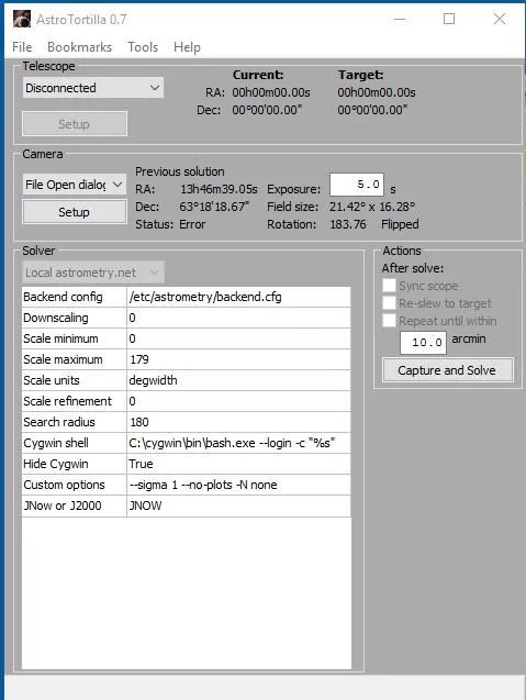
- Nach 32 Sekunden liefert AstroTortilla mit dem Solver “Local astrometry.net” ein Ergebnis:
- RA: 13h 46m 39,05s Dec: 63° 18′ 18,67″ Exposure 5.0 s Field size: 21,42° x 16,28° Rotation: 183,76 Flipped
Abbildung 1: Platesolving mit Astro Tortilla (pCloud: AstroTortilla01.jpg)
Vergleiche: Abbildung 10
AstroTortilla01
Ein wunderschönes Ergebnis. Mit den Koordinaten ist wohl die Bildmitte gemeint. Aber welche Sterne sind den nun tatsächlich auf dem Foto?
Tutorial (Imaging): Setting up and Using AstroTortilla for Plate Solving
Copyright: Light Vortex Astronomy
AstroTortilla is one of those programs that may seem overly complicated to set up and start using, hence this short tutorial for those interested. It is however a program that once you start using, you will not regret having spent the time to install it and set it up. Best of all, AstroTortilla is completely free and works wonders for plate solving. For those unaware, plate solving is a process by which software checks your astrophotograph for star patterns and determines what it is you are actually looking at. Why is this in any way important, though? Simple – when you tell your telescope to go to a deep space object, it will go to it but will probably miss and not have your chosen object centred in view. Of course, a decent three-star goto alignment prior to slewing to your target removes quite a lot of the error but:
- The goto alignment will very seldom provide you with perfect goto accuracy.
- Why bother picking multiple stars and aligning them perfectly when you would rather spend the time actually imaging your target?
It is here that AstroTortilla excels. You set up your telescope and CCD camera, you send your telescope to your target and then tell AstroTortilla to plate solve. It will capture an image with your CCD camera, analyse it to check where you are actually aiming and then slew your telescope to remove the goto error and centre your target. It can even iterate through this process until your target is very precisely centred within a chosen margin of error (default is 1 arcminute). I tend to only need a single iteration to get my target perfectly centred. If you are interested, you will need to sort out a couple of things beforehand:
- Your mount must be controlled via a laptop and the likes of EQMod or other such ASCOM software, through an EQDirect USB interface. This is paramount as AstroTortilla needs to interface with your mount directly via ASCOM.
- Download the latest version of AstroTortilla for free from this link.
Please feel free to ask questions or leave comments via the comments section on the bottom of this page. Alternatively, you may send me a quick message through the About page, e-mail me via the button on the top-right of this website or contact me through forums or Facebook.
Tabelle 1: Inhaltsverzeichnis des Tutorials
|
Contents
|
1. Installing AstroTortilla
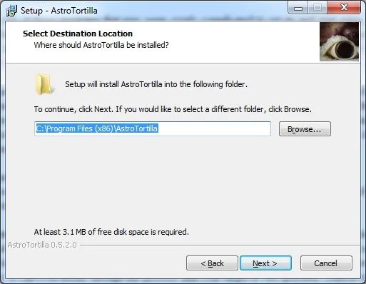
Though it may sound silly going through the installation process, there is a bit we need to pay close attention to. Choose to install AstroTortilla to the default directory.
Abbildung 2: AstroTortilla Installation Destination (pCloud: AstroTortilla_setting_up_astrotortilla_-_1.1.jpg)
AstroTortilla Installation: Destination
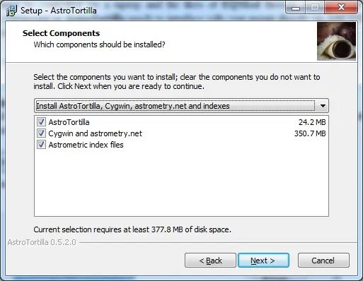
As we are installing everything from scratch, leave the default option “Install AstroTortilla, Cygwin, astrometry.net and indexes” selected with everything checked.
Abbildung 3: AstroTortilla Select Components (pCloud: AstroTortilla_setting_up_astrotortilla_-_1.2.jpg)
AstroTortilla Components
If it were all installed but we simply wanted additional astrometric index files (these are the reference files that contain the star patterns to match up against your captured images and astrometric index files are different for different fields of view), we would select “Install additional astrometric index files”.
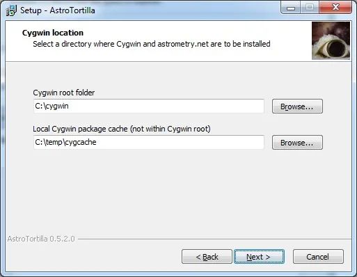
It is important to install Cygwin (part of AstroTortilla’s package) to its default directory.
Abbildung 4: AstroTortilla: Cygwin location (pCloud: AstroTortilla_3927552_orig.jpg)
AstroTortilla Cygwin Location
Abbildung 5: AstroTortilla Index selection (pCloud: AstroTortilla_6754082_orig.jpg)
Vergleiche: Abbildung 9
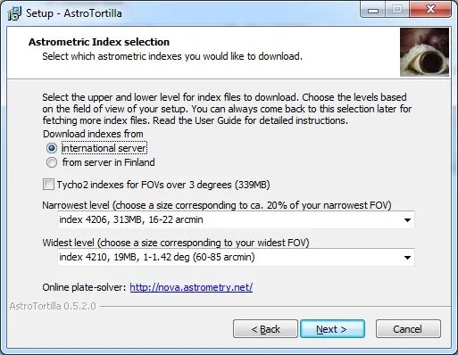
AstroTortilla: Index SelectionWe now reach the important stage that we need to carefully consider.
You may have multiple telescopes and multiple CCD cameras. Matching these up will naturally produce different fields of view and if we want to install AstroTortilla armed with all required astrometric index files to work on all your combinations, we will need to figure out the fields of view produced by your narrowest-field setup and your widest-field setup. For example, say you have two telescopes and one CCD camera. One produces a wide-field and another a narrow-field. It is easy to figure out the range of astrometric index files required. In order to calculate the fields of view, we can use the free, online Sky at Night Field of View Calculator.
Abbildung 6: Field of View Calculator (pCloud: AstroTortilla_2763989_orig.jpg)
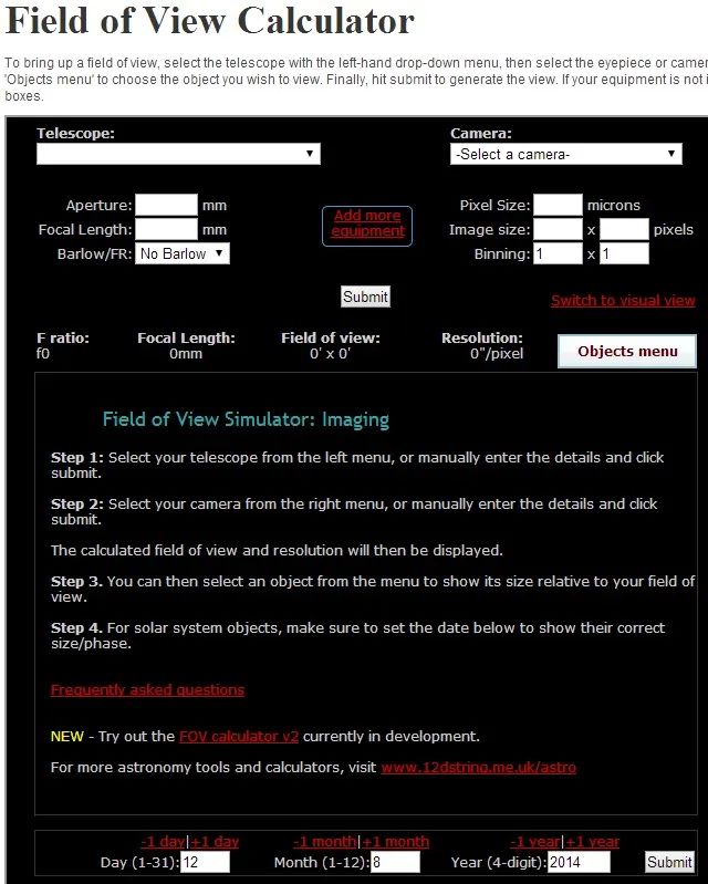
AstroTortilla: Field of View CalculatorYou may find your telescope and CCD camera listed and therefore you can simply select these (do verify the details are correct!). My CCD camera, the QSI 660wsg-8, was not on the list and neither were my telescopes. So, I therefore verified the details of my CCD camera with the manufacturer, QSI, and then manually entered my first telescope’s details (having measured the exact focal length beforehand – see another tutorial).
Abbildung 7: Field of View (pCloud: AstroTortilla_4668114_orig.jpg)
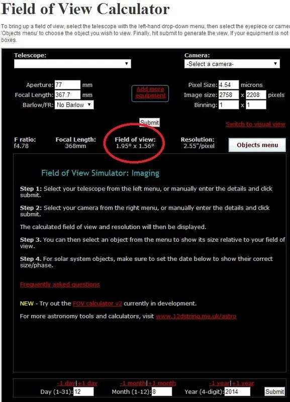
AstroTortilla: Field of ViewI note that my Borg 77EDII with my QSI 660wsg-8 yields a field of view of 1.95 degrees x 1.56 degrees.
Now I enter my second telescope’s details.
Abbildung 8: Field of View (pCloud: AstroTortilla_2351746_orig.jpg)
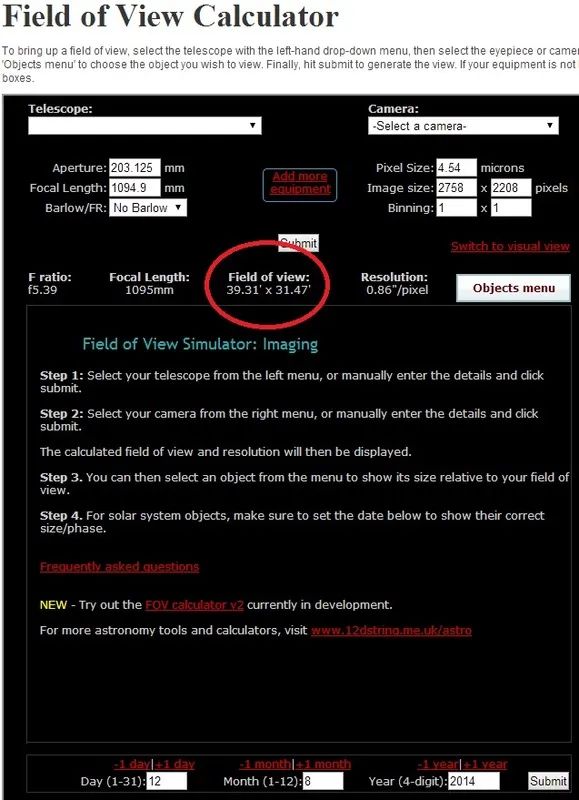
AstroTortilla: Field of View 2Finally, I note that my Altair Astro 8″ RC with my QSI 660wsg-8 yields a field of view of 39.31 arcminutes x 31.47 arcminutes.
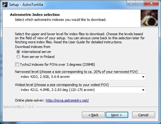
Now we return to the AstroTortilla installation process. First I select my widest field of view. We always use the biggest number of the two. My widest field of view is 1.95 degrees x 1.56 degrees, so I take the field of view number to be 1.95 degrees (the largest number). From the astrometric index files list on Widest level, I select:
The range of 2 – 2.83 degrees clearly covers my 1.95 degrees. Now for the narrowest field of view. The installation suggests we select about 20% of our narrowest field of view, so let us do that. My narrowest field of view is 39.31 arcminutes x 31.47 arcminutes, so I take the field of view number to be 31.47 arcminutes (the smallest number). 20% of it is 6.294 arcminutes. From the astrometric index files list on Narrowest level, I select:
index 4203, 2.5GB, 5.6-8 arcmin
This range clearly covers 20% of my narrowest field of view, 6.294 arcminutes.
Abbildung 9: AstroTortilla Index selection (pCloud: AstroTortilla_9919543_orig.jpg)
Vergleiche Abbildung 5: AstroTortilla_6754082_orig.jpg
AstroTortilla: Index Selection 2
Please note the installation will actually download these two astrometric index files and every other one in-between them. Checking the file sizes, the astrometric index files for narrower fields of view are quite large and the entire download probably sums up to about 4.9GB in total for my telescopes and CCD camera. Your astrometric index files will probably differ from mine.
If indeed you only have one telescope and one CCD camera, then it is simpler. For example, let us say that I only have the Borg 77EDII telescope and QSI 660wsg-8 CCD camera. We calculated the field of view to be 1.95 degrees x 1.56 degrees for this setup. We therefore take our widest field of view here to be 1.95 degrees and the narrowest to be 1.56 degrees. 20% of the narrowest is then 0.312 degrees (or 18.72 arcminutes, multiplying by 60) and we have our numbers for selecting appropriate astrometric index files.
Once you have adequately selected your needed astrometric index files, proceed with the installation and finish it. No doubt the downloading of astrometric index files will take a while, depending on your Internet connection with the server.
2. Setting up AstroTortilla with Optimum Settings for Fast Plate Solving
When you first run AstroTortilla, it might look intimidating and perhaps even unrefined. It is however very powerful and you need not do much to configure it and get it running.
Abbildung 10: AstroTortilla (pCloud: AstroTortilla01.jpg)
Vergleiche: Abbildung 1
Let us first summarise the sections of this window.
Under Telescope, we connect to the telescope mount and once connected, you are shown your current telescope position in the night sky as well as your intended target. Basically when you issue a goto command for the telescope to slew to your target, it will most assuredly miss and you will notice the difference under Current and Target.
Under Camera, we connect to the CCD camera via compatible software such as Nebulosity, MaxIm DL, Backyard EOS, etc. We can also ask AstroTortilla to control the CCD camera directly via ASCOM or in fact, select File Open dialog and select an image that we have taken by our own means (without asking AstroTortilla to do it itself automatically). Here we also set the desired exposure time. Unless you are currently using a narrowband filter, 10 seconds usually suffices. If you are using a narrowband filter, it may be a good idea to switch to a regular LRGB filter. If you are using a refracting telescope and are already focused with say, Hydrogen-Alpha (or Sulphur-II), using Red would be a close match for focus (Green is a good match for Oxygen-III).
AstroTortilla will work even if you are slightly out of focus anyway. Using a regular LRGB filter, which is broadband, will allow a lot more light through and will produce more stars for plate solving in a shorter exposure time (this is particularly true for Luminance). Once plate solved, you can always switch back to your narrowband filter for imaging without ever touching the focus.
Under Solver, we can customise a couple of settings, and this is what we will do first and foremost. These settings tell AstroTortilla what field of view we are actually dealing with (to give it a head-start in plate solving and allowing it to take much less time), how many degrees off from your target you wish to look at, the noise tolerance, etc.
Under Actions, we set off AstroTortilla to do its job. It is of utmost importance that we always check Sync scope and Re-slew to target as these will make sure AstroTortilla does the job of centering your target in view and adding a sync point to EQMod (like a star alignment point) to correct future slewing accordingly. You could also of course check the third option Repeat until within and enter an amount of arcminute tolerance. Please note this will cause AstroTortilla to iterate through the process at least twice (first time to perform the initial error correction and second time to check resulting accuracy), with more iterations possible depending on how far off you are from your target after the first correction. The Capture and Solve button of course, sets it all off to do its magic.
The first thing we will do is change some settings in AstroTortilla, under the Solver section. Since I have two telescopes and one CCD camera, I have two setups I can possibly use. I will therefore create two settings files, one for each setup, so that in the future I can load up the one I need and set it off quickly.
The first settings we will change are Scale minimum and Scale maximum. These are where you tell AstroTortilla the minimum and maximum field of view possible. Let us say I am using my Altair Astro 8″ RC telescope first. This provided a field of view of 39.31 arcminutes x 31.47 arcminutes with my CCD camera. We will work with degrees rather than arcminutes and therefore dividing these numbers by 60 gives us the field of view to be 0.655 degrees x 0.525 degrees. We note then that the maximum is 0.655 degrees and the minimum is 0.525 degrees. We need not be 100% accurate (these numbers are a little rounded off) and so I will enter 0.5 in Scale minimum and 0.7 in Scale maximum. You may enter rounded off numbers as long as Scale minimum is below your actual minimum and Scale maximum is above your actual maximum.
Abbildung 11: AstroTortilla: Scale min&max (pCloud: AstroTortilla_5681440_orig.jpg)
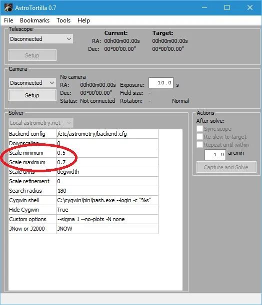
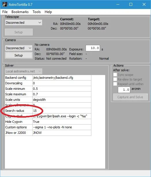
AstroTortilla: ScaleI will leave degwidth in Scale units as we are entering everything in degrees. Now we must edit Search radius. The default value of 180 is way too high. This means AstroTortilla will search 180 degrees around your target. This is quite simply savage as though we will miss the target, we will not miss it by 180 degrees! To be safe though, we will set 15 degrees, so I enter 15 here. Please keep in mind this value if it turns out AstroTortilla is not successfully plate solving your images. You may want to first try increasing it to 30 or even 45 just in case. You should never need to go higher than 45. Similarly, you may never be as far off as 15 degrees and so you may decrease it and test it out. As long as it plate solves, the lower this value is, the faster it will work.
Abbildung 12: AstroTortilla Search Radius (pCloud: AstroTortilla_4239689_orig.jpg)
AstroTortilla: Search Radius
Finally, we will alter Custom options. The first option that is there by default is particularly important, –sigma 1. This defines the noise tolerance in analysing your captured image for plate solving. The default value of 1 is very, very small and pretty much any speck on your image may be considered a star. Even with a cooled CCD camera, this is certainly not the case and in fact, we do not want too many stars to be considered for plate solving as it would take ages. For a 10 second exposure (without a narrowband filter in place!), a much better value is something like 50 to 70. In fact, any value between 50 and 100 is good depending on the number and brightness of the stars in your field of view. This value is balanced out with exposure time, as you would imagine. I would set it to 70 and then just alter exposure time to suit. We leave the parameters –no-plots and -N none there but add two more. We will reiterate to AstroTortilla the field of view we expect. For this, we use the options -H and -L, which are widest field of view and narrowest field of view, respectively. I will stick to the same values as with Scale minimum and Scale maximum and therefore enter -H 0.7 -L 0.5 to the end of Custom options, after adding a space.
There are two more Custom options that are particularly interesting. These help speed up plate solving and are in some way related to one another. They are -r and –objs. The former, -r, need only be added as that. This command instructs AstroTortilla to sort the stars in order of brightest first, therefore allowing AstroTortilla to optimise the plate solving process as it starts with the brightest stars in your image. The second option to help speed up plate solving is rather to ensure that if it is going to fail, that it fails quicker rather than keeping you waiting. The parameter –objs command must be accompanied by a number, e.g. –objs 100. What this command does is instruct AstroTortilla to use a maximum of 100 stars for the plate solving (the developers generally recommend between 100 and 200 stars). After having sorted them in brightest-first, it seems like a good idea to restrict how many AstroTortilla should use as if it fails after the first and brightest 100, for example, there is a very, very good chance it will simply fail altogether. At that point of course you would adjust other parameters such as your exposure time. Please be aware however that these options are not always best. Sometimes you may want to include more stars than 100 or you may not want to restrict the number of stars used. This could be due to persistent plate solving failures. Feel free to remove the –objs command if you feel it necessary, though the -r command tends to be a good idea to leave active.
Abbildung 13: AstroTortilla Custom Options (pCloud: AstroTortilla_5863500_orig.jpg)
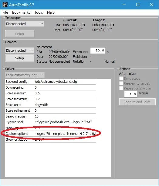
AstroTortilla: Custom Options
Due to the length, you cannot see the entire Custom options line in the above screenshot. For reference, it reads:
–sigma 70 –no-plots -N none -H 0.7 -L 0.5 -r –objs 100
Nebulosity 3 for my imaging, with my QSI 660wsg-8 CCD camera. Also, I will be binning my images in 2×2 when it comes to plate solving as this will brighten the image significantly in the exposure time set and it will bring out more stars as well. Binning has the additional benefit that the file size and resolution is reduced by a factor of four, meaning that AstroTortilla will be much faster at processing the image and plate solving it. To set the software, camera and binning mode I will use, I simply select Nebulosity 2/3 from under Camera and then click Setup. Here, I select QSI 500/600 from the list, verify the directory for Nebulosity 3 is correct and select 2 in Binning.
Users of a DSLR, which cannot bin images, would benefit from setting Downscaling to 1 under Solver. This will at least downscale the image in order to make it faster to process and plate solve. Binning is most definitely preferable to downscaling simple because binning downscales by its very nature but at the same time, produces an image with a lot more brightness and more stars picked up. Downscaling alone simply makes the image smaller, with no added benefit to the stars detected.
Abbildung 14: AstroTortilla Camera Setup (pCloud: AstroTortilla_8864129_orig.jpg)
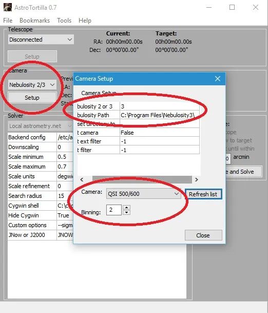
AstroTortilla: Camera Setup Nebulosity
Abbildung 15: AstroTortilla: Save Settings (pCloud: AstroTortilla_4482496_orig.jpg)
Vergleiche Abbildung 19 AstroTortilla_6379424_orig.jpg
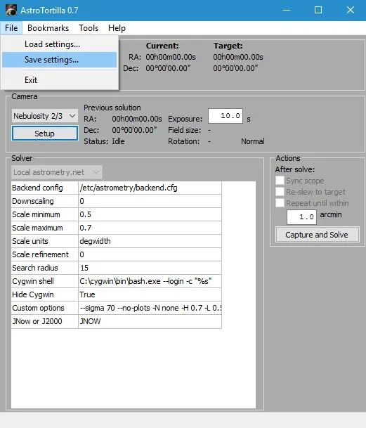
AstroTortilla: Save Settings
Abbildung 16: AstroTortilla: Save Settings (pCloud: AstroTortilla_8117221_orig.jpg)
Vergleiche Abbildung 20 AstroTortilla_3770875_orig.jpg
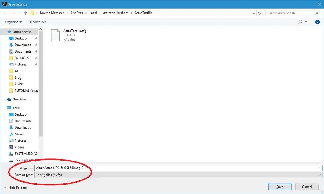
AstroTortilla Save Settings FileNow to customise AstroTortilla to my Borg 77EDII telescope with the QSI 660wsg-8 CCD camera. We note the field of view was calculated to be 1.95 degrees x 1.56 degrees. This will again define our values of Scale minimum and Scale maximum. We therefore enter 1.5 for Scale minimum and 2.0 for Scale maximum. Again, we are rounding off slightly below the actual minimum and above the actual maximum.
Abbildung 17: AstroTortilla Scale (pCloud: AstroTortilla_915917_orig.jpg)
Siehe Abbildung 11: AstroTortilla_5681440_orig.jpg
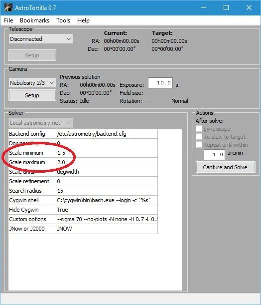
AstroTortilla: Scale 2We will leave Search radius at 15, like before, and –sigma 70 in Custom options (for noise tolerance). I of course will alter the -H and -L options to enter the same values as Scale minimum and Scale maximum. -r and –objs 100 are added on as well.
Abbildung 18: AstroTortilla Custom Options (pCloud: AstroTortilla_8621068_orig.jpg)
Siehe Abbildung 13: AstroTortilla_5863500_orig.jpg
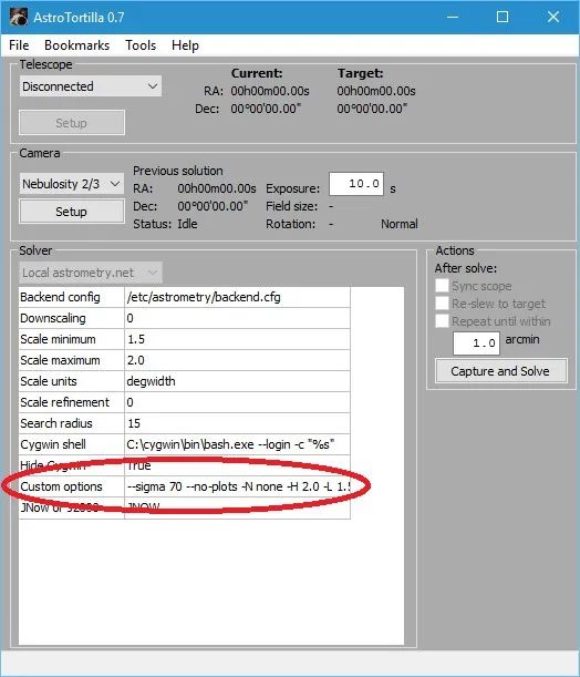
AstroTortilla: Custom Options 2Due to the length, you cannot see the entire Custom options line in the above screenshot. For reference, it reads:
–sigma 70 –no-plots -N none -H 2.0 -L 1.5 -r –objs 100
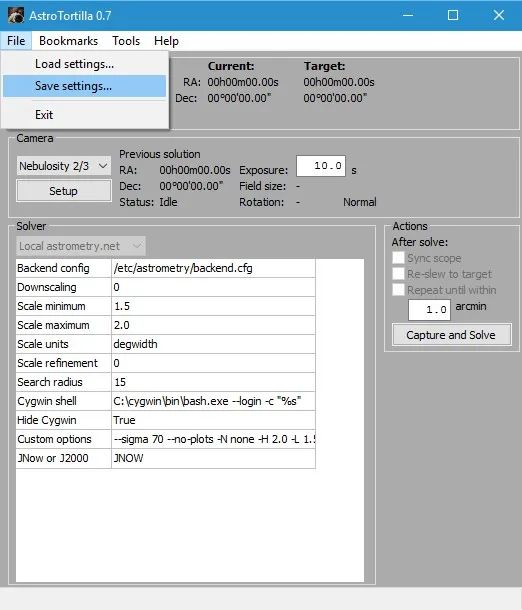
The same settings under Camera are kept, using Nebulosity 2/3, the QSI 500/600 camera and Binning at 2 (for me personally, of course). I now save these settings to a new settings file, naming it appropriately.
Abbildung 19: AstroTortilla: Save Settings (pCloud: AstroTortilla_6379424_orig.jpg)
Vergleiche Abbildung 15 AstroTortilla_4482496_orig.jpg
AstroTortilla Save Settings 2
Abbildung 20: AstroTortilla Save Settings File 2 (pCloud: AstroTortilla_3770875_orig.jpg)
Vergleiche Abbildung 16 AstroTortilla_8117221_orig.jpg
AstroTortilla Save Config File 2
I have now customised AstroTortilla for both my telescopes and their resulting fields of view. Depending on my imaging setup on a particular night, I can load up the appropriate settings file. These settings optimise the plate solving process to make it significantly faster and always yield a solution. You may need to alter exposure time to suit if a solution is not found when plate solving or it seems to be taking too long. For reference, plate solving should normally take under 2 minutes to perform in total.
If for any reason the stars in your images are not coming out round and plate solving is therefore failing (optical defects, collimation, focus, etc), you can add another Custom option to relax AstroTortilla’s restriction on what constitutes a star. The command for this is -c, which needs to be followed by a value. As a default, AstroTortilla uses -c 0.01 but if you wish to relax this a little, you can add -c 0.02 to your Custom options. If you increase it, do so by very small amounts, like -c 0.02.
3. Using AstroTortilla for Plate Solving
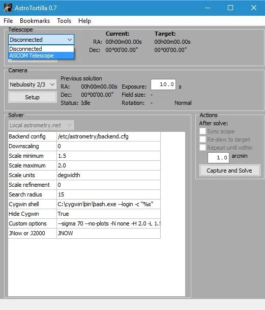
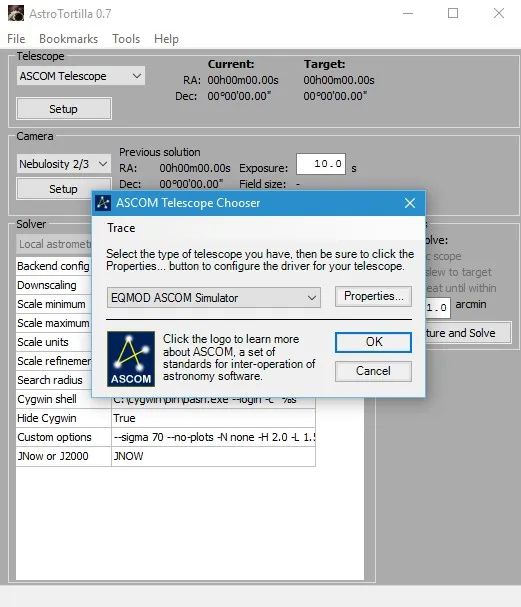
With the appropriate settings file loaded (for the imaging setup being used), the first thing we need to do is connect to our telescope mount via ASCOM. So, we select ASCOM Telescope from the list at the top and then confirm via the ASCOM dialog that pops up (I am using the simulator for this tutorial!).
Abbildung 21: AstroTortilla: ASCOM Telescope (pCloud: AstroTortilla_1842666_orig.jpg)
AstroTortilla: Connect ASCOM Telescope
Abbildung 22: AstroTortilla: ASCOM Telescope Chooser (pCloud: AstroTortilla_5503543_orig.jpg)
AstroTortilla: ASCOM Telescope Chooser
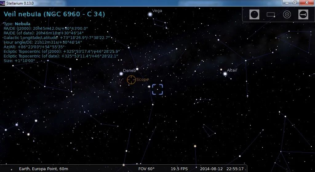
Once connected to the telescope, I issued a goto command in Stellarium to slew the telescope to the Veil Nebula.
Abbildung 23: AstroTortilla: Goto Veil Nebula (pCloud: Stellarium_1474865_orig.jpg)
AstroTortilla: Goto Veil Nebula
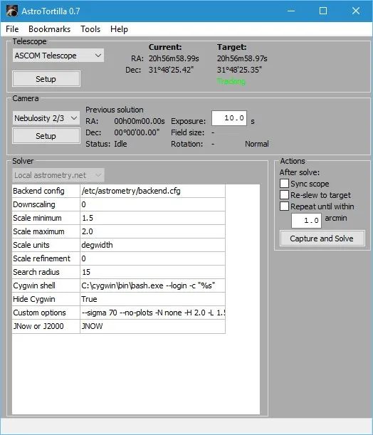
Abbildung 24: AstroTortilla Current/Target (pCloud: AstroTortilla_2629214_orig.jpg)
AstroTortilla Current/Target
With the telescope on target, you can gauge an idea of the error under Telescope within AstroTortilla (comparing Current to Target co-ordinates). In a real-life situation, the difference here will be much bigger (remember I am using the simulator for this tutorial!). With Tracking displayed under Target, we are ready for plate solving.
Now we will need to connect to the CCD camera. You have a choice of what to do here. Open your program and connect to the CCD camera within the program. Once connected to the CCD camera, select the program from the list in AstroTortilla if you have not done so beforehand (when you created your settings file).
It is important to start the program and connect to your CCD camera beforehand as AstroTortilla will issue commands to the program itself to start capture, after which it will download the resulting image and start the plate solving. If your program is not listed on AstroTortilla or for some reason is not working as intended, you can always capture the image yourself within your program and save it somewhere. Then in AstroTortilla, select File Open dialog for Camera and later when we start plate solving, it will ask you to open the image file. This ensures AstroTortilla is very universal. You can also of course, connect to your CCD camera directly by selecting ASCOM Camera and then selecting the appropriate driver from the list, which will be installed if you have used your CCD camera in the past. If you are having AstroTortilla capture and download the image itself (and not providing one via the File Open dialog), set an appropriate exposure time as well. 10 seconds tends to be very suitable and you are advised not to make exposures too long, though you can also do 20 seconds or so. Under 1 minute is always good.
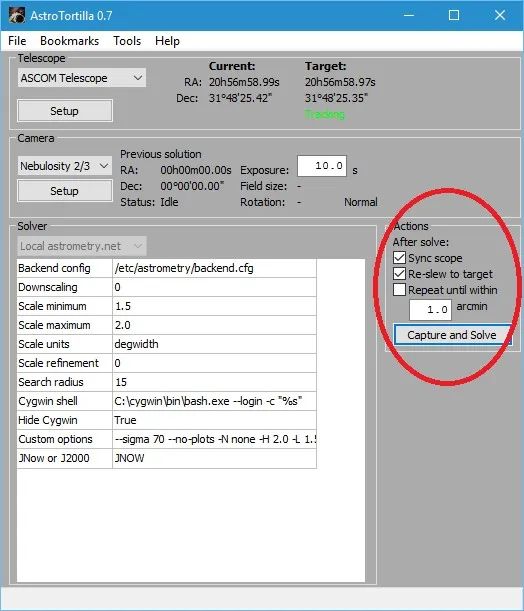
Before starting plate solving, check Sync scope and Re-slew to target under Actions. The first ensures an alignment point is added to the likes of EQMod (this acts like a star alignment, which makes future goto commands more precise). The second ensures the target is physically centred after AstroTortilla plate solves, which is the main idea behind us even using AstroTortilla to begin with.
Abbildung 25: AstroTortilla: Capture and Solve (pCloud: AstroTortilla_5584514_orig.jpg)
AstroTortilla: Capture and Solve
To start plate solving, all we need to do now is click the Capture and Solve button and watch it happen. In my experience, one plate solving iteration centers my objects perfectly but if you want to be very precise about it, check the third option Repeat until within and enter a respective accuracy in arcminutes. Please note that this will cause the plate solving process to be repeated again and again until the desired accuracy is achieved. At the very minimum, two plate solving processes will occur – the first to perform the initial centering to your target and the second to check that it is within desired accuracy. Speaking from personal experience, I find my target is always precisely centred in the field of view of my camera without using the Repeat until within option, with a single plate solve.
In any case, when happy, click Capture and Solve. AstroTortilla will first capture your image, download it and start plate solving (if you chose to provide an image file yourself via File Open dialog, it will just ask you for the image file). The plate solving process starts by searching its astrometric index files (the ones you downloaded for installation) for a match, calculating how far off you are, slewing your telescope appropriately and syncing the difference as a goto alignment point in EQMod. Subsequent iterations of this process are up to you (dependent on your chosen accuracy for repetition).
This concludes how to use AstroTortilla. It really is that easy and after having customised it for your possible telescope setups, plate solving should be a fast process. Do make sure you play around with exposure time if a solution is not yielded with a 10 second exposure but remember that under 1 minute is good. Too long an exposure time will basically take longer to capture and will not really be necessary for plate solving. You can of course play around with the –sigma value here as well. Decrease it to include more stars and increase it to reject dimmer stars.
4. Further Optimising Plate Solving Speed
After you have used AstroTortilla to plate solve successfully a couple of times, you will notice a pattern. Since you have a large number of astrometric index files downloaded and stored for plate solving, AstroTortilla will look through them all until it finds a match to your exposure and then does its magic. If you look closely, it will seem that it will always find a match for your particular telescope-camera pair in one astrometric index file, or two or three, but never seems to make use of the other astrometric index files. This is normal. During the installation, a lot of astrometric index files were downloaded as per your field of view limitations. Most of these however, are not needed (as evidenced by your plate solving successes). We can use this fact to produce a further speed optimisation to plate solving.
To accurately determine which astrometric index files are useful, one must use the Log Viewer by going to the Tools menu and clicking Log Viewer. This will open a new, small window on the side.
Abbildung 26: AstroTortilla: Tools -> Log Viewer (pCloud: AstroTortilla_1079311_orig.jpg)
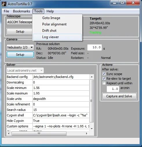
AstroTortilla: Tools -> Log Viewer
Abbildung 27: AstroTortilla Log Viewer Window (pCloud: AstroTortilla_1219258_orig.jpg)
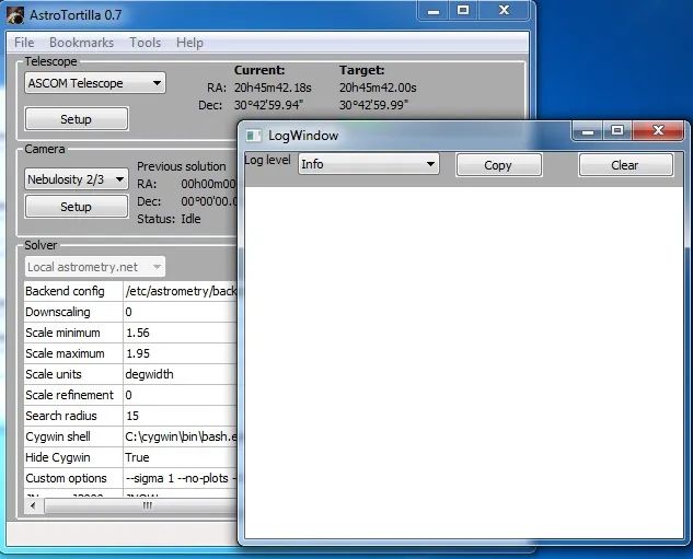
AstroTortilla LogViewer Window
Keep Info selected from the list and now carry out your plate solving as usual. The events that appear and disappear quickly on the very bottom of AstroTortilla will be listed in sequence in the the Log Viewer. You can scroll through them to see what has happened over time. You can also scroll right to see which astrometric index file was being looked at, at the time.
Abbildung 28: AstroTortilla Log Viewer (pCloud: AstroTortilla_1333089_orig.jpg)
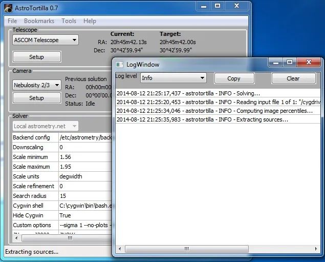
AstroTortilla Log Viewer
Abbildung 29: AstroTortilla LogWindow (pCloud: AstroTortilla_5341826_orig.jpg)
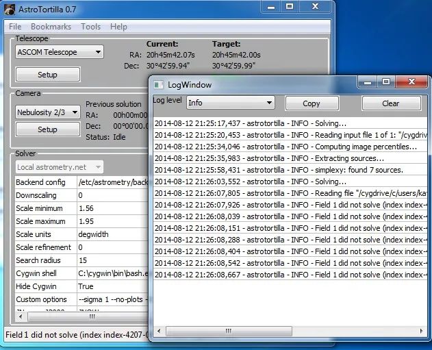
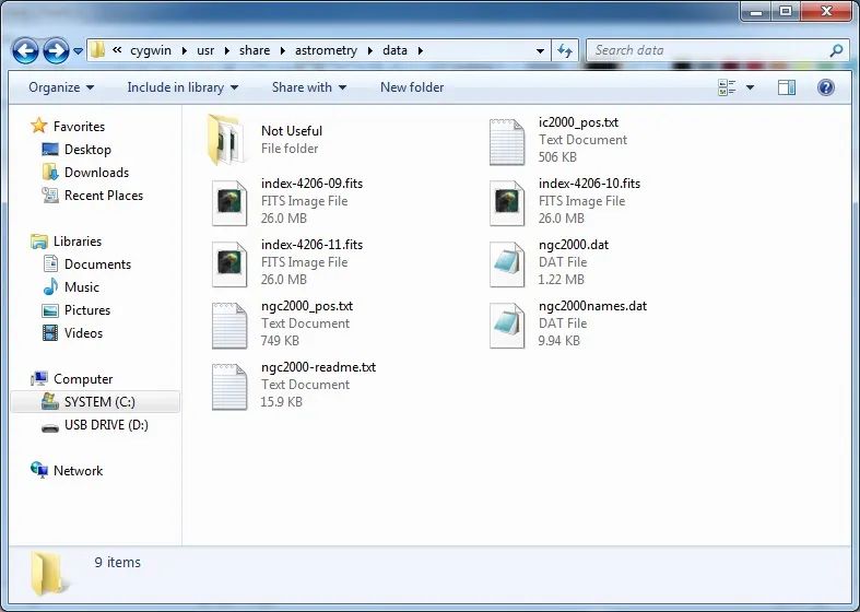
AstroTortilla LogWindow filledEventually it will successfully plate solve and it will tell you so, showing you which astrometric index file was the successful one in matching your exposure. Take note of the astrometric index file name. Please do remember that from one target to the next, it may end up plate solving successfully with another astrometric index file, though usually this is an adjacent one (e.g. it may normally succeed using index-4206-11.fit but another night on another region of the night sky it will succeed using index-4206-10.fit). Normally it appears two or three astrometric index files does the job for a particular telescope-camera pair. Do note that, as in my case, if you use different telescope-camera pairs, you will no doubt have a couple of useful astrometric index files per telescope-camera pair.Once you have determined which astrometric index files do it for you, you can physically move the unused ones out of the usual folder so that they are missing during plate solving and thus AstroTortilla does not waste time in looking through them (as they are useless to you anyway). To access the astrometric index files you have, assuming you installed everything in its default directories, go to the following folder:
C:\cygwin\usr\share\astrometry\data
Abbildung 30: AstroTortilla: Folder for Index files (pCloud: AstroTortilla_6838327_orig1.jpg)
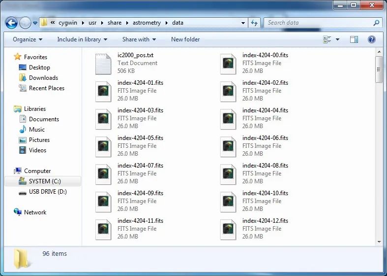
AstroTrortilla Folder for Index Files
There are clearly a good number of astrometric index files there, as per my installation of AstroTortilla. Now, let us say we determined that actually only the following were useful for me:
- index-4206-09.fit
- index-4206-10.fit
- index-4206-11.fit
It is then a simple process of selecting all the other astrometric index files (just the files with .fit as file extensions) and moving them to a custom sub-folder I made, named Not Useful.
Abbildung 31: AstroTortilla: Index Files (pCloud: AstroTortilla_7677656_orig.jpg)
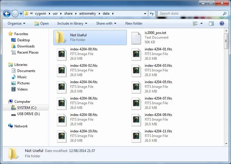
AstroTortilla Not Usefull Index Files
Abbildung 32: AstroTortilla Index Files (pCloud: AstroTortilla_9821654_orig.jpg)
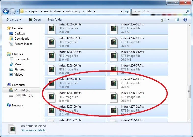
AstroTortilla Index Files
Abbildung 33: AstroTortilla Index Files (pCloud: AstroTortilla_6006521_orig.jpg)
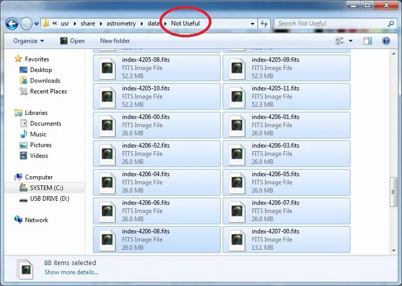
AstroTortilla Index Files Not Useful
Abbildung 34: AstroTortilla Index Files (pCloud: AstroTortilla_9351208_orig.jpg)
AstroTortilla Index Files Useful
Above I demonstrate the created Not Useful folder, selection of all astrometric index files except the useful ones, moving the selected ones to the Not Useful folder and then how the only available astrometric index files are now the ones I deemed useful. By experience, this should make a plate solve that usually takes around 30 seconds (as reported by AstroTortilla) succeed in just under 5 seconds. That is certainly a big deal. The reason the astrometric index files are not just simply deleted is because we may actually need them in the future, which brings us to the caveat of this optimisation technique
The caveat is that if you do not experiment with plate solving enough to know which astrometric index files are really useful, you may end up moving a useful one inadvertedly and thus causing plate solving to fail on that particular target. This is a simple thing to fix however. Simply access the Not Useful folder and move one astrometric index file back over. Choose one that is above or below the ones you currently have available. For example, if I have the above three but plate solving failed, I would choose to move back either index-4206-08.fitor index-4207-00.fit. I would move only one and retry plate solving until it succeeds as there is no point in deviating too far from the usually useful astrometric index files or introducing too many new ones into our availability pile.
One final note is that since you are already in the folder storing all your .fit astrometric index files, you may as well back them up somewhere. If you choose to re-install AstroTortilla for any reason, you can skip ahead and not download any astrometric index files. Instead, you can copy-paste your backup of all your .fit files in place. This saves a lot of time when it comes to installing AstroTortilla.
5. Things to Try when Plate Solving Fails to Centre the Target or Fails Completely
Though this tutorial has thus far covered what astrometric index files to download and how to correctly configure AstroTortilla, there are always reports of users who experience nothing but failed plate solve events, or not centering the target as perfectly as intended. If AstroTortilla is succeeding at plate solving and appears to not really centre your target, instead placing it consistently off-centre, then your problem is related to different epochs being used by the mount and AstroTortilla. The epochs users can select from most software are J2000 and JNow. By default, AstroTortilla uses the JNow epoch.
Abbildung 35: AstroTortilla: Epoch (pCloud: AstroTortilla_5343608_orig.jpg)
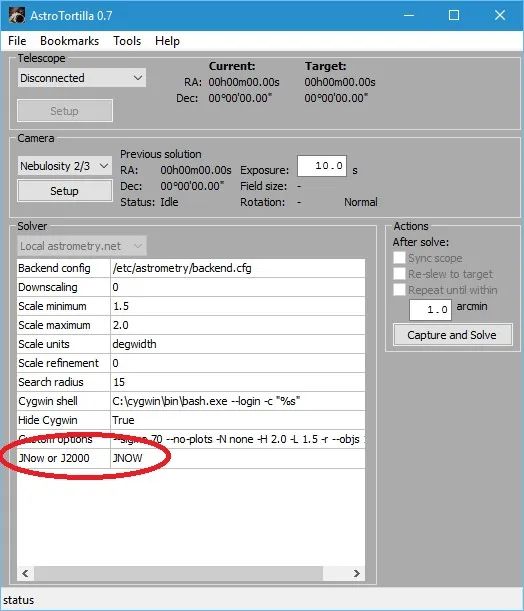
AstroTortilla: Epoch JNow
This is fine so long as your mount is also using JNow, for example. If you are using EQMod to control your mount, then you can set the mount epoch you want under Driver Setup in the EQModToolbox.
Abbildung 36: AstroTortilla Epoch in EQMOD (pCloud: EQASCOM-01.jpg)
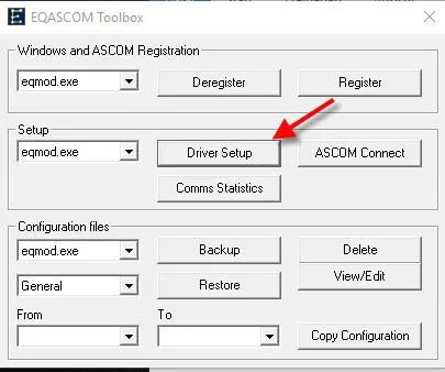
AstroTortilla: Epoch EQMOD Setup
Abbildung 37: AstroTortilla Epoch EQMOD Setup (pCloud: AstroTortilla_2928268_orig.jpg)
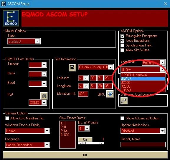
AstroTortilla: Epoch EQMOD Setup
The key is simply making sure both your mount’s and AstroTortilla’s epochs agree. This way the goto error correction command sent by AstroTortilla to the mount is interpreted as intended. There is no specific advantage to using JNow over J2000 however, so do not stress about this.
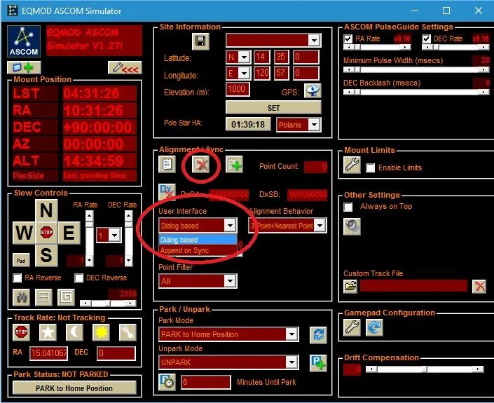
What happens if AstroTortilla appears to be successfully plate solving your target but then gets stuck on the “Re-centering“process and your mount does nothing? This is a common issue that tends to be fixed by parking the mount, switching it off, switching it back on and trying again. However, at times the problem is stubborn, or you may not want to park the mount and cycle its power. This is fixed by stopping EQMod from storing the star alignment points when AstroTortilla sends the Sync command. All you have to do is select Dialog Based under User Interface in Alignment / Sync. You should also click the Clear Align Data button to delete all star alignment points saved thus far.
Abbildung 38: AstroTortilla EQMOD SYNC (pCloud: AstroTortilla_5495740_orig.jpg)
AstroTortilla SYNC EQMOD
The default setting on User Interface in Alignment / Sync on EQMod is Append on Sync. This setting adds new star alignment points when an ASCOMSync command is sent by software such as AstroTortilla (or Stellarium through StellariumScope, for example). The setting Dialog Based allows users to manually enter star alignment point data. This ignores all ASCOMSync commands and therefore fixes the “Re-centering“ getting stuck issue in AstroTortilla.
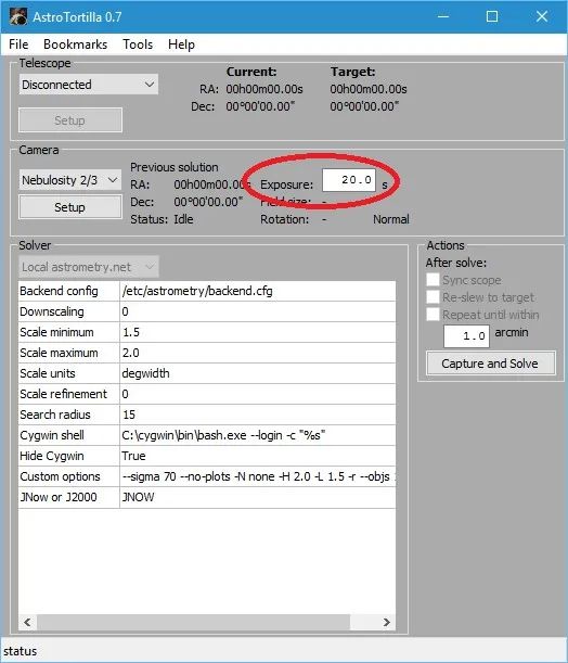
The above covers if AstroTortilla plate solves but does not successfully centre your target. However, what if AstroTortilla does not plate solve at all? The common error here is “Field 1 did not solve”, usually after several minutes of frustrating wait. The first thing to try is to increase the exposure time on AstroTortilla (or the image capture software you are using). First however, make sure you are not using a narrowband filter in front of your sensor (if using a monochrome CCD camera).
Abbildung 39: AstroTortilla Exposure Time (pCloud: AstroTortilla_3984117_orig.jpg)
AstroTortilla Plate Solving Exposure Time
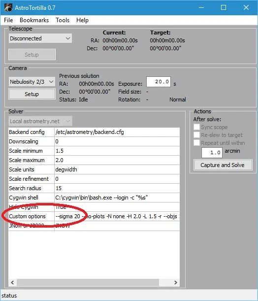
I have personally always found 20 seconds to suffice with a Luminance filter, looking through telescopes that range between f/4.5 and f/5.5 focal ratio. If this does not work, you can try lowering the value on the –sigma parameter under Custom options. By lowering –sigma, more objects detected in your exposure will be treated as stars for comparison with the astrometric index files. If your current value is 70, you could try values such as 50, 30, 20, etc. Avoid values lower than about 10 however.
Abbildung 40: AstroTortilla Custom Options: Sigma (pCloud: AstroTortilla_4490212_orig.jpg)
AstroTortilla Custom Options Sigma
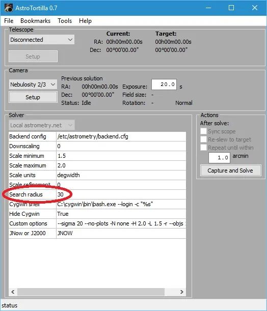
If your exposure time has been increased and your –sigma value has been decreased but you are still not getting plate solving to work, you may wish to expand the Search radius. 15 should work perfectly well but this can be increased to 30 or even 45. You should not need to go this high but there is nothing wrong with values of 45 or lower.
Abbildung 41: AstroTortilla: Search Radius (pCloud: AstroTortilla_5329735_orig.jpg)
AstroTortilla Solver Search Radius 30
In the unfortunate scenario that you are still having problems plate solving with AstroTortilla, it is time to look at the astrometric index files again. By default, AstroTortilla downloads the 4200 series of astrometric index files, which are based on the 2MASS star catalog. However, in particular for wide-field setups, the 4100 series of astrometric index files can be much better. These are based on the Tycho2 star catalog. Downloading these can be done by running the AstroTortilla installer again, selecting only to install additional astrometric index files.
Abbildung 42: AstroTortilla Additional Index Files (pCloud: AstroTortilla_5562525_orig.jpg)
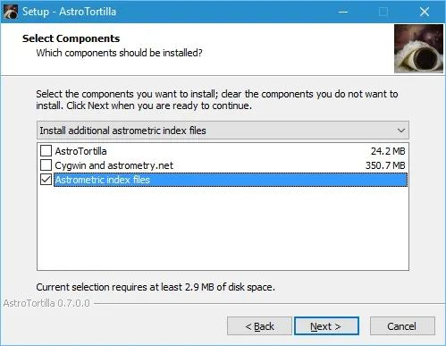
AstroTortilla Additional Index Files
On the next screen, you need to check to enable the option ”Tycho2 indexes for FOVs over 3 degrees (339MB)”.
Abbildung 43: AstroTortilla Tycho2 Index Files (pCloud: AstroTortilla_6437877_orig.jpg)
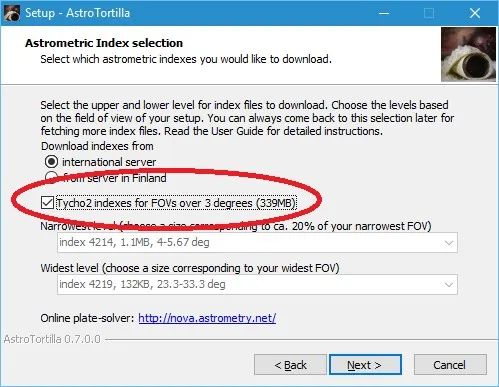
AstroTortilla Tycho2 Index Files
Enabling this option will disable the astrometric index file selection below it. Do not worry. Continuing the setup will actually download the entire set of 4100 series of astrometric index files, at only about 339MB. Once these are downloaded, it is worth trying plate solving once again.
If it works, you could then refine your settings again. Perhaps with the 4100 series of astrometric index files downloaded, you can use a Custom options setting of –sigma 70 and Search radius of 15. Though not required to download new astrometric index files (as you can use the AstroTortilla setup to do this), you can access these files directly at the Astrometry.net addresses for the 4100 series and 4200 series astrometric index files (click links). At these addresses, you may download the individual astrometric index files and place them in their required folder:
- C:\cygwin\usr\share\astrometry\data
Comments
(Feb 24, 2016) kayronjm (mod) said:
@Steve Mills,Hi Steve,I see what you mean. You want to download FURTHER astrometric index files in addition to the ones you already have. To do this, simply run AstroTortilla’s installer again, but don’t uninstall what you have. Run the installer and when it asks what components you wish to install, simply select “Install additional astrometric index files”. In the next screen, simply set what you want OVERALL, even if you already have some. Choose the range you now want to have, and the installer will check what files you already have and only download the missing ones (the new files). That’s it – once done, you’re good to go. Remember to re-configure AstroTortilla with the new combination’s settings for FOV.
(Feb 24, 2016) Steve Mills said:
Once you enter the info on the setup screen, how do you get back to that screen to re-enter DIFFERENT “widest” and “narrowest” data if you change scopes and/or cameras?
(Dec 28, 2015) Magnus Kvant said: